浅析跳表性能缺陷
由于redis和leveldb的兴起,跳表走入了大众的实现
相对红黑树而言,跳表非常容易理解,使其成为了红黑树的常见替代
刚好我在理解2-3-4树的时候写了红黑树,顺便写一个跳表来pk一下性能
结果是我万万没想到的:
在单线程下,跳表的性能几乎全方位被红黑树碾压
这里特意提及了单线程,是因为多线程下的leveldb的无锁跳表显然性能会比加锁的红黑树更好
然而在单线程下,如果追求极限性能,红黑树总是会比跳表更好
为了测试结果有说服力,我引入了redis原生的t_zset.c来进行性能测试
redis跳表微调
支持多种数据结构
源码:https://github.com/tedcy/algorithm_test/blob/master/order_set/t_zset.h
为了多种数据结构的测试,zskiplist相关数据结构和zsl相关函数都改成了模板
由于跳表使用了C99的flexible array members,这在C++会遇到一些小问题
因此我对zslCreateNode做了简单修改,在非pod类型时显式进行placement new调用构造函数
1 | template <typename T> |
支持find
原生的跳表是没有find功能的,只有通过rank来查询数据,或者通过score来获取rank,我对zslGetRank进行简单修改以支持find
1 | template <typename T> |
红黑树改为顺序统计红黑树
源码:https://github.com/tedcy/algorithm_test/blob/master/order_set/rb_tree.h
如果不支持相同的数据操作,那么性能对标没有任何意义
因此红黑树需要在支持getRank等操作下进行测试
红黑树对某个节点getRank类似于遍历前驱节点,这显然是\(O(n)\)的时间复杂度
可以进一步对这个简陋的算法进行优化
因为红黑树的顺序和中序遍历结果一致,对某个节点而言,左子树的全部节点都在它前面
所以在简陋算法前驱遍历的过程中如果节点存在左子树,则可以直接跳过所有左子树的节点,从而获得类似于\(O(\log n)\)的时间复杂度
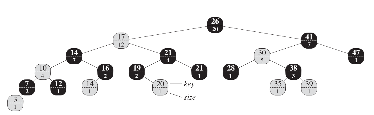
跳过左子树的方法是对每个子树维护一个x.size = x.left.size + x.right.size +1,在发现左子树时,直接rank += x.left.size + 1即可
如下图:
插入操作修改
插入节点有两部分
- 记录插入过程中向下查找时经过的全部节点,如果插入成功,那么对它们size+1
1 | Node* findParent(Node* cur, const KeyT &key) { |
- 旋转时,更新将变为子节点的原父节点的size,并且更新新父节点的size
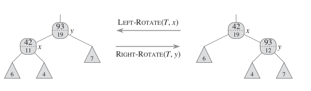
伪代码:
1 | /*左旋*/ |
源码:
1 | //turn curParent to be cur Node left child |
删除操作修改
删除节点也有两部分
- 找到真正删除的后继节点deleteNextNode后,从其到根节点的size全部-1
deleteNextNode本身也需要size-1,将其视为一个没有size的虚节点,在后续删除的旋转操作中才可以正确进行计算
1 | ... |
- 旋转,插入操作时已经修改了这一部分代码
根据值查询排名(getRank)
正如上文所述,这是一个找前驱节点的过程,在这个过程中,如果存在左子树,那么rank += (cur->left->size + 1)即可
然后继续findParentPrev寻找向上的前驱节点
1 | Node* findParentPrev(Node* cur) { |
根据排名查询值(getByRank)
对一个节点cur进行rank查找,可以查看是否rank == cur->left->size + 1
如果rank < cur->left->size + 1,说明可以在他的左子树中寻找rank
否则可以在他的右子树中寻找rank - cur->left->size - 1
这个算法可以直接用递归来写,因为是尾递归
1 | Node* getByRank(Node* cur, int rank) { |
性能测试
测试对象
我一共测试了6种数据结构,数据量都为100万
RBTreeBase<T, false>为不带rank功能的红黑树RBTreeBase<T, true>为带rank功能的红黑树SkipList<T>为我自己写的不带rank功能的跳表ZSet<T>为redis跳表,带rank功能,除了forward节点以外还带了一个反向的backward节点- 红黑树天生支持逆序遍历,从这个角度看,完整结构的跳表性能下降会很明显
- 下面的测试也论证了这一点,
ZSet<T>作为完整体,各项性能会比SkipList<T>下降了20%左右,使其不堪的性能雪上加霜
set<T>为标准库红黑树unordered_set<T>为标准库哈希表- 纯粹好奇性能差距放在这里,由于支持的操作不同,不存在比较意义
测试源码
https://github.com/tedcy/algorithm_test/blob/master/order_set/test.cpp
常规测试
插入(insert)测试
1 | RBTreeBase<int, false> insert: Cost 605 ms |
不带rank功能的红黑树和不带rank的跳表比快了27%
带rank功能的红黑树和redis跳表比快了38%
从另外一个角度来看,红黑树带rank只损失了8%的性能,跳表带rank则损失了22%的性能
红黑树在插入性能上好于跳表
查询(find)测试
1 | RBTreeBase<int, false> find: Cost 519 ms |
不敢置信,跳表的查询性能居然只有红黑树的一半
从另外一个角度来看,红黑树带rank没有损失性能,跳表带rank则损失了17%的性能
删除(erase)测试
1 | RBTreeBase<int, false> erase: Cost 623 ms |
不管是红黑树还是跳表,删除操作都需要先找到待删除节点
因此删除性能是查询性能的延伸,可以看到在删除性能上,跳表依然落后于红黑树,但是比起查询操作差距有所缩小
遍历(range)测试
最出乎我意料之外的就是遍历时间复杂度了
1 | RBTreeBase<int, true> range: Cost 91 ms |
可以看到跳表领先的时间相当少,甚至使用string后,随着内存消耗的上升,跳表的时间消耗被反超了!
红黑树的遍历是每个节点访问两次,差不多是\(2O(n)\)的时间消耗,居然还能领先于跳表\(O(n)\)的时间消耗?!
接着看相对于list的时间消耗,跳表的性能差的让人大跌眼镜
而众所周知跳表是加了索引的链表结构,那么为什么会相差如此大的幅度呢?
使用perf进行了简单分析
1 | Performance counter stats for process id '31531': ZSet |
可以看到perf结果中ZSet和list的L1访问大致相当
ZSet的LLC-loads 19674183是list的LLC-loadss 2313517的850%,也就是ZSet的内存访问大部分都穿透到L3缓存中去了
而L1的性能是L3的10倍,因此性能下降的主要原因就在这里了
使用perf record具体看一下引起cache-references(略大于LLC-loads+LLC-stores)的部分
1 | Samples: 80 of event 'cache-references', 99 Hz, Event count (approx.): 16134258 std::_Function_handler<void (), testRangePerformanceNest<ZSet<int>, std::__cxx11::list<int, std::allocator<int> > >()::{lambda()#1}>::_M_invoke /root/algorithm_test/order_set/out.exe |
可以看到不管ZSet还是list都100%是操作寄存器操作,因此我认为是ZSet的局部性过差导致了遍历性能的下降
我猜测局部性过差的原因是ZSet的内存消耗远高于普通链表,而且跳表随机level产生的节点在内存中不如链表这么规则,导致无法很好的进行缓存读取优化
顺序统计(Rank)测试
根据值查询排名(getRank)测试
1 | RBTreeBase<int, true> getRank: Cost 808 ms |
对跳表而言,getRank的算法和搜索算法是几乎一样的,因此有相近的时间消耗
而对红黑树而言,getRank类似于遍历前驱节点,在这个过程中如果节点存在左子树,则可以直接跳过所有左子树的节点,从而获得类似于\(O(\log n)\)的时间复杂度。相比find而言,会有更高的常数项时间复杂度消耗,然而即使是这样,性能依旧好于跳表
根据排名查询值(getByRank)测试
1 | RBTreeBase<int, true> getByRank: Cost 775 ms |
依旧是红黑树好过跳表
根据排名上下限遍历(rangeByRank)测试
在100万元素中随机上下限rank进行遍历,并重复1000次
1 | RBTreeBase<int, true> rangeByRank: Cost 25799 ms |
rangeByRank是getRank和rangeByRank的结合
这是我的一个工程场景:
数据存在多个索引,查询时无法完全匹配索引,此时通过最左前缀匹配分析最优索引,随后对索引进行遍历对数据一一匹配
类似于sql中explain多个索引时需要回表的场景
在这种场景下,红黑树略差于跳表
别人的性能测试
我一度认为是我测试的代码有问题,找了一些别人的测试结果
他测试了查询和更新结果,红黑树的性能平均是跳表的1.5倍,倒是和我测试的结果相近
又在查阅了一些资料以后,发现也有人和我有相同的疑惑
Skip lists, are they really performing as good as Pugh paper claim?
在Stack Overflow上的这个贴主实现的AVL树暴打了跳表,所以他发帖询问
最高评分的回答是这样的:
Times have changed a bit since William Pugh wrote his original paper. We see no mention in his paper about the memory hierarchy of the CPU and operating system which has become such a prevalent focus today (now often equally as important as algorithmic complexity).
His input case for benchmarking had a measly 2^16 elements, and hardware back then typically had, at most, 32-bit extended memory addressing available. This made the size of a pointer half the size or smaller than what we're used to today on 64-bit machines. Meanwhile a string field, e.g., could be just as large, making the ratio between the elements stored in the skip list and the pointers required by a skip node potentially a lot smaller, especially given that we often need a number of pointers per skip node.
C Compilers weren't so aggressive at optimization back then with respect to things like register allocation and instruction selection. Even average hand-written assembly could often provide a significant benefit in performance. Compiler hints like
registerandinlineactually made a big deal during those times. While this might seem kind of moot since both a balanced BST and skip list implementation would be on equal footing here, optimization of even a basic loop was a more manual process. When optimization is an increasingly manual process, something that is easier to implement is often easier to optimize. Skip lists are often considered to be a lot easier to implement than a balancing tree.So all of these factors probably had a part in Pugh's conclusions at the time. Yet times have changed: hardware has changed, operating systems have changed, compilers have changed, more research has been done into these topics, etc.
大意是说Pugh论文只有6万多个元素的测试集,另外当时的指针比现在小得多,但是字符串的大小是一样的,使得当时跳表所需的指针比率小得多
另外当时的编译器还不够智能,因此更复杂的AVL需要更复杂的优化才能得到更好的性能
在30年的后的今天,不同大小的数据集,不同硬件,不同编译器当然会带来完全不一样的结果
接着最高评分的回答写了一些代码优化来提升性能,甚至做了一些作弊手段来提高性能,才使得跳表性能略好于红黑树
所以他最后总结:
Today the benefits of locality of reference dominates things to a point where even a linearithmic complexity algorithm can outperform a linear one provided that the former is considerably more cache or page-friendly. Paying close attention to the way the system grabs chunks of memory from upper levels of the memory hierarchy (ex: secondary stage) with slower but bigger memory and down to the little L1 cache line and teeny register is a bigger deal than ever before, and no longer "micro" if you ask me when the benefits can rival algorithmic improvements.
The skip list is potentially crippled here given the considerably larger size of nodes, and just as importantly, the variable size of nodes (which makes them difficult to allocate very efficiently).
算法的性能现在很大程度的取决于L1缓存的命中率,跳表的节点size太大了,并且不是固定大小,使得很难高效的去分配他们。
这倒是我和在跳表遍历的性能测试中得到的结论一致,跳表在访问的节点时的局部性实在是太差了。
跳表的时间复杂度分析
常规测试时间复杂度分析
遍历时间复杂度分析
跳表毫无疑问是\(O(n)\)
红黑树是\(2O(n)\),这个证明非常简单:
先找到最小节点,这个复杂度是\(O(\log n)\)
然后依次找后继节点,后继节点的查找有两种模式
向下:如果存在右子节点,说明下一个节点是右子树的最左节点
- 因此找到右子节点的向下最左节点
向上:如果不存在右子节点,说明当前节点已经是某子树的最大几点,因此需要向上遍历,直到找到当前子树作为左子树的父节点
- 因此找到第一个子节点是父节点的左子节点,使得子节点代表的子树成为一颗左子树
如图,绿色是遍历时经过节点:
顺带一提,后继的向下向上和前驱的向上向下刚好的逆向的过程
graph TB subgraph id[ ] subgraph 后继向下,前驱向上 c3((2))---d3((...)) c3((2))---e3((5)) d3((...))---f3((...)) d3((...))---g3((...)) e3((5))---h3((4)) e3((5))---i3((...)) h3((4))---j3((3)) h3((4))---k3((...)) i3((...))---l3((...)) i3((...))---m3((...)) style c3 fill:#9f9,stroke:#333,stroke-width:4px style e3 fill:#9f9,stroke:#333,stroke-width:4px style h3 fill:#9f9,stroke:#333,stroke-width:4px style j3 fill:#9f9,stroke:#333,stroke-width:4px end subgraph 后继向上,前驱向下 a4((7))---e4((2)) e4((2))---h4((...)) e4((2))---i4((4)) h4((...))---j4((...)) h4((...))---k4((...)) i4((4))---l4((...)) i4((4))---m4((6)) a4((7))---b4((...)) b4((...))---c4((...)) b4((...))---d4((...)) style a4 fill:#9f9,stroke:#333,stroke-width:4px style e4 fill:#9f9,stroke:#333,stroke-width:4px style i4 fill:#9f9,stroke:#333,stroke-width:4px style m4 fill:#9f9,stroke:#333,stroke-width:4px end end在遍历的过程中,红黑树的每一个节点在向下时经过一次,再向上时又会经过一次,因此这一部分的时间复杂度是\(2O(n)\)
综上\(2O(n)\)+\(O(\log n)\)约等于\(2O(n)\)
但是红黑树在遍历的过程中可以用到计算机和编译器对局部性的优化,因为节点大小固定且较小,且遍历过的节点后续还会经过一次
跳表的节点恰恰相反,因此遍历性能和红黑树没差别,测试时string类型还会更差一些
插入,删除,查询时间复杂度分析
由于插入性能和删除性能都依赖查询性能,因此以查询性能作为切入点进行时间复杂度分析,就能得到两者插入删除查询的时间复杂度下限了
大致可以搞明白跳表比起红黑树差在哪里
插桩分析
我在代码里插了桩,来计算跳表和红黑树的平均查询次数
1 | Node* find(const KeyT& key) { |
1 | Node* find(const KeyT& key) { |
插入4个元素后,进行查询,由于跳表的插入level是随机的,因此额外插桩构造一个平均情况下的跳表
由于P=0.25的时间复杂度和P=0.5时大致相当,因此如下进行构造
1 | switch (key) { |
最终得到的总比较次数,红黑树是8,而跳表为16
也就是查询一次跳表的比较次数是红黑树的两倍,这倒是符合之前的性能测试
查询每个元素分析
4个元素{1,2,3,4}的红黑树的如图
graph TB
    subgraph id[ ]
        subgraph 红黑树
        a2((2))---b2((1))
        a2((2))---c2((3))
        c2((3))---e2((nil))
        c2((3))---f2((4))
        style f2 fill:#f9f,stroke:#333,stroke-width:4px
        end
    end
对查询来说:
元素1需要2次比较
元素2需要1次比较
元素3需要2次比较
元素4需要3次比较
然后来看下跳表的查询插桩日志吧:
1 | find|v=1| |
根据日志进行可视化整理:
- 红黑树结构如下:
1 | level 3:head-------------------4 |
具体查询过程如下:
=线代表查询过程
1 | 元素1需要3次比较: |
可以看到,每个元素比较次数远超红黑树
每一层都需要find next来达到下一层,可以认为日志find next是爬层高,日志find element是爬链表
爬层高的时间复杂度\(O(\log n)\)
爬链表的时间复杂度也是\(O(\log n)\)
因此时间消耗是红黑树的两倍
时间复杂度分析
上述的插桩时间复杂度分析虽然可视化效果好易于理解,但是并不严谨,因此来看下论文是如何推理时间复杂度的
论文将查询节点的过程反向回溯
- 如果节点没有上一层指针,那么正向搜索过程就不可能经过上一层指针,所以只能由左节点遍历过来
- 例如上文举例{1,2,3,4}元素的跳表,需要寻找元素3,他只有1层,从元素3第1层回溯,那只能从元素2第1层遍历过来
- 如果节点有上一层指针,那么正向搜索过程就不可能从左节点遍历过来,最差情况下也会从上面的节点下降到当前节点
- 例如上文举例{1,2,3,4}元素的跳表,需要寻找元素3,他只有1层,当前回溯节点的是元素1第1层,如果元素1有上一层,就至少会从上一层查询next失败以后,才会下降到当前层
对照刚才的查询过程
1 | 元素3查询过程: |
因此,假设从一个层数为i的节点x出发,需要回溯k层
- 如果节点x无i+1层指针,那么需要向左走,这种情况概率为1-p
- 如果节点x有i+1层指针,那么需要向上走,这种情况概率为p
用\(C(k)\)表示向上攀爬k个层级所需要走过的平均查找路径长度
那么可以得到:
- \(C(0) = 0\)
- \(C(k) = (1-p)(C(k) + 1) + p(C(k-1) + 1)\)
- 化简:
- \(C(k) = (C(k) + 1) - (pC(k) - p) + (pC(k-1) + p)\)
- \(C(k) = C(k) + 1 - pC(k) + pC(k-1)\)
- \(pC(k) = 1 + pC(k-1)\)
- \(C(k) = \dfrac{1}{p} + C(k-1)\)
- \(C(k) = \dfrac{k}{p}\)
- 化简:
对一个节点数为n的跳表而言,一共需要爬\(\log \frac{n}{p} - 1\)层
因此跳表的平均查找路径长度大致为\(\dfrac{\log_{\frac{1}{p}} n - 1}{p}\)
由于爬到顶层以后还需要向左走一些步数,但是这个可以忽略不计,严格推导可以看原论文
将\(p = 0.25\)代入,得\((\log_4n - 1) * 4\),也就是\((\log_2n - 1) * 2\)
而红黑树的查询时间复杂度显然为\(O(\log_2n)\)
因此可见跳表的查询性能是红黑树的一半
而跳表和红黑树插入和删除都是基于查询后做一些操作,由于红黑树的后续操作最坏时间复杂度\(O(\log_2n)\),总体最坏是\(2O(\log_2n)\),和跳表查询的时间复杂度一致
因此红黑树的插入删除不可能比跳表的插入删除性能更差
总结
综上所述,在单线程下,跳表的性能几乎全方位被红黑树碾压
另外,完全体的跳表为了支持顺序统计加入span后,理解难度甚至高于红黑树:代码量膨胀了一倍,虽说代码量和算法复杂程度不一定成正比,但是更长的代码显然带来更多需要理解的细节。红黑树看着代码多,但是有一半的代码和另一半基本一致,是镜像场景的代码重写一遍。
更别说完全体的跳表为了反向遍历加入了backward指针以后,在内存的节省上优势也减少了:在选择P为0.25时,平均每个节点需要2.33个指针,而红黑树需要左右父节点3个指针。
因此我认为,在单线程下,跳表是红黑树的下位替代。
单线程只有在有限的场景下,才需要选择跳表(例如redis,如下)
redis为什么使用跳表?
这里是作者回复
antirez on March 6, 2010 | root | parent | next [–]
There are a few reasons:
They are not very memory intensive. It's up to you basically. Changing parameters about the probability of a node to have a given number of levels will make then less memory intensive than btrees.
A sorted set is often target of many ZRANGE or ZREVRANGE operations, that is, traversing the skip list as a linked list. With this operation the cache locality of skip lists is at least as good as with other kind of balanced trees.
They are simpler to implement, debug, and so forth. For instance thanks to the skip list simplicity I received a patch (already in Redis master) with augmented skip lists implementing ZRANK in O(log(N)). It required little changes to the code.
About the Append Only durability & speed, I don't think it is a good idea to optimize Redis at cost of more code and more complexity for a use case that IMHO should be rare for the Redis target (fsync() at every command). Almost no one is using this feature even with ACID SQL databases, as the performance hint is big anyway.
About threads: our experience shows that Redis is mostly I/O bound. I'm using threads to serve things from Virtual Memory. The long term solution to exploit all the cores, assuming your link is so fast that you can saturate a single core, is running multiple instances of Redis (no locks, almost fully scalable linearly with number of cores), and using the "Redis Cluster" solution that I plan to develop in the future.
原因1是和b树对比,正如刚才所述,选择P为0.25时,和红黑树相比在内存上也是略有领先的,作为一个内存数据库,确实是选择跳表的理由
原因2是遍历性能至少和其他类型平衡树一样好,这不算选择跳表理由
原因3是容易实现,很容易扩展支持ZRANK,那基于红黑树的顺序统计树也容易实现,所以也不算选择跳表的理由
所以redis选择跳表的唯一理由就是省内存了,而作为一般的后端开发者,基本上都可以拿空间去换时间,毕竟平台的cpu资源总是比内存要更紧张一些
参考资料
红黑树改造为顺序统计树
- https://en.wikipedia.org/wiki/Order_statistic_tree
- 算法导论--动态顺序统计与区间树
- 在二叉树中找到一个节点的后继节点
- 学习笔记—寻找二叉树的前驱节点和后继节点
跳表时间复杂度分析
-
时间复杂度分析写的不错,为什么要用跳表这个分析的不够深入
https://lotabout.me/2018/skip-list/
时间复杂度写的凑活,参考资料挺全的
https://oi-wiki.org/ds/skiplist/
oi-wiki,复杂度证明比其他的会严格一些,最严格的话还是得看原论文
https://www.51cto.com/article/669167.html
解释了早期redis随机跳表层数的写法原理,但是在后续版本redis已经改掉了,因为跨平台的支持不好