快速排序细节分析
在翻看C++标准库源码的时候,突然发现std::sort的实现和我想的很不一样,并不是简单的快排
在查询了一些资料以后,大致搞明白了这个introsort的原理
这篇写的很好:知无涯之std::sort源码剖析
另外就是STL源码分析那一本写的很好,不是本文的重点,简单过一下,我的gcc版本是5.4.0
introsort原理
1 | __introsort_loop(_RandomAccessIterator __first, |
introsort先在__introsort_loop中进行传统快排的分区算法和递归,每一轮递归减少__depth_limit
当初始值为lg(__last - __first) * 2,也就是2lgN的__depth_limit归零后,判断快排可能进入了劣化局面,可能会退化为O(N^2)的时间复杂度
因此使用__partial_sort也就是堆排序,最差时间复杂度为O(nlgn)
然后当递归到__last - __first <= _S_threshold(值为16)
那么结束递归,调用__final_insertion_sort做插入排序,因为插入排序在元素较少或大致有序时速度较快
讨论的重点在std::sort使用的快排
std::sort使用的快排
1 | template<typename _RandomAccessIterator, typename _Compare> |
我遇到了几个问题,为什么pivot的值进行了一定的选择?
为什么分区算法是双指针,而算法导论上是单指针,另外双指针都没有判范围,这样不会跑挂吗?
根据一些资料查询,这里使用的是三点取中Hoare分区算法
那么回顾一下算法导论的快排,对比一下区别吧
算法导论的快排
单指针分区算法又叫Lomuto分区算法,非常的简单易懂
1 | int quick_sort_partion(vector<int> &nums, int start, int end) { |
Hoare分区算法
双指针算法又叫Hoare分区算法,是设计快排的大佬设计的分区算法
在std::sort的unguarded_partition中,last--没和first++放在一起,是因为last代表着区间的后一个元素,因此需要提前进行一次last--
将last--后置以后,大概是如下算法
1 | int random_quick_sort_partion(vector<int> &nums, int start, int end, int pivotIndex) { |
这里有几个问题:
1 为什么不需要边界检测?
2 为什么start == end的时候需要break?
3 为什么随机pivot不能取start?
4 为什么返回start作为分隔?end可不可以?
5 为什么Hoare分区后递归的区间和Lomuto分区算法不一样?
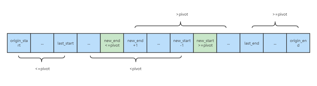
回答这些问题前,先看下这个图
这个图绘制了即将跳出循环的情况
origin_start代表random_quick_sort_partion的参数start,origin_end同理
last_start代表上一轮循环交换时start停留的位置,last_end同理
new_start代表本轮循环start会在哪里停留,new_end同理
为什么不需要边界检测?
以start为例进行分析
假设当前是第一轮循环,那么最坏情况下
new_start会停在pivot的位置上假设当前是第N轮循环,那么N-1次循环的时候,
last_start和last_end交换的以后,nums[last_end,origin_end]这一段必然>=pivot了那么最坏情况下
new_start会停在last_end上
end同理,因此不需要边界检测
end的时候需要break?
首先给反例
假设给一个有序自增且不重复的序列
pivot_index取origin_end,那么第一轮循环,new_start在[0,origin_end]都不符合要求,会直接跑越界pivot_index取origin_start同理,new_end会朝着起点方向越过0跑越界如果start == end的时候break,就能防止越界
其次
start == end的时候,表示这是同一个值,此时swap是冗余操作
为什么随机pivot不能取start?
即使start == end的时候break,随机pivot也不能取start
假设给一个有序自增且不重复的序列,当pivot_index取start的时候,第一轮循环new_start停在origin_start,new_end在[origin_start + 1,origin_end]都不符合要求,也停在origin_start
此时分区算法返回的q为origin_start,那么下一轮quick_sort的递归,会分别计算[origin_start,q - 1] 和 [q,origin_end]
也就是[origin_start,origin_start - 1] 和 [origin_start, orgin_end],后者和本轮递归的范围一致,会导致无限递归无法收敛
为什么返回start作为分隔?end可不可以?
可以的,观察图片可以得到结论new_start停在>=pivot的值上,new_end停在<=pivot的值上
对start作为分隔来说
由于[
origin_start,new_start- 1]一定<=pivot,所以可以作为一半的分隔而[
new_end,origin_end] > pivot,new_start>=new_end,因此[new_start,origin_end]作为子集一定也>pivot,所以可以作为另外一半的分隔简单的来说
new_start可能>pivot,因此在分区算法的右边,返回start时为[start, q - 1],[q, end]对end作为分隔来说
由于[
new_end+ 1,origin_end]一定>=pivot,所以可以作为一半的分隔而[
origin_start,new_start] < pivot,new_end<=new_start,因此[origin_start,new_end]作为子集一定也<pivot,所以可以作为另外一半的分隔简单的来说
new_end可能<pivot,因此在分区算法的左边,返回end时为[start, q],[q + 1, end]另外,返回end时,随机pivot不能取end:
假设给一个有序自增且不重复的序列,当
pivot_index取end的时候,第一轮循环new_end停在origin_end,new_start在[origin_start,origin_end- 1]都不符合要求,也停在origin_end此时分区算法返回的q为
origin_end,那么下一轮quick_sort的递归,会分别计算[origin_start,q] 和 [q + 1,origin_end]也就是[
origin_start,origin_end] 和 [origin_end+ 1,orgin_end],第一次递归和本轮递归的范围一致,会导致无限递归无法收敛
因此如果返回end可以这样实现代码
1 | void random_quick_sort_imp(vector<int> &nums, int start, int end) { |
为什么Hoare分区后递归的区间和Lomuto分区算法不一样?
核心原因是因为Hoare分区算法只保证大于pivot和小于pivot的值分隔开,不考虑=pivot的值的位置,当向下递归时,总能保证这一轮递归=pivot的值会放置在该放的位置
而Lomuto分区算法会保证=pivot值在分区完成后一定在他该在的位置,这增加了很多计算量
这也是Hoare分区算法的优势,在序列存在大量相同值时,性能会比Lomuto分区算法好得多
当然这也增加了边界计算时的复杂性,也就是3.3和3.4看到的,会有bad_case导致递归无法收敛而无限递归
new_end最大为1
这是观察图片可以得到的一个额外的有趣结论
由于[last_start + 1, new_start - 1]都小于pivot
而 [new_end + 1, last_end - 1]都大于pivot,由于new_start >= new_end
那么在new_start和new_end之间的数[new_end + 1, new_start - 1]既要大于pivot又要小于pivot
这显然是不可能的,因此new_start最多比new_end大1
我想这也是这个算法性能高的原因,我一开始还担心start++和end--的循环里不做start和end的大小的边界校验,会浪费很多性能
性能测试
测试环境
1 | gcc: gcc version 5.4.0 20160609 (Ubuntu 5.4.0-6ubuntu1~16.04.10) |
随机数测试:
100w数据,[0, INT_MAX]全随机
1 | Lomuto分区算法: |
有序数测试:
1w数据,[0, 9999]有序
数据量较少,因为部分测试算法在该用例下时间复杂度过高跑太久了
1 | Lomuto分区算法: |
各个算法在随机数上的情况差不多
但是在顺序数的情况下,Lomuto分区算法在有序数上性能下降明显,Hoare分区随机算法会好很多
pivot三点取中Hoare分区算法的性能会比Hoare分区随机算法低(前者算法胜在稳定,不会因为随机运气特别差而撞到O(n^2))
而标准库算法在pivot三点取中Hoare分区算法的基础上进一步优化,性能快得多,几乎赶上了Hoare分区随机算法,也就是理想情况下的O(nlgn)复杂度的时间消耗
Hoare分区算法的局限性
根据上面的分析,Hoare算法在各种场景下都完爆了Lumoto算法,那Lumoto算法的意义是什么?
当分区时选到的pivot有重复数字,需要pivot的重复数字在分区后强制有序时,Hoare算法就不能用了,这个场合也很常见,那就是快速选择算法
快速选择算法
用于解topK问题,标准库算法对应std::n_element
快速选择算法只需要找到序列中排第几位的数字,因此不需要完全有序
假设要找到从0开始下标为k的数字
和二分查找的逻辑类似,每次分区后:
当
k = 分区算法返回值q,那么直接返回- 当
k < 分区算法返回值q,那么n_element(nums, start, q - 1) 当
k > 分区算法返回值q,那么n_element(nums, q+1, end)
这要求返回q时,这个q所在位置和最终结果位置是一致的
举个例子,Hoare算法后分区的序列为11211,k=4,返回的q为4,然后就直接返回结果为1,但答案应该是2。这里的问题就在于1没有完全顺序。如果用Lumoto算法后,分区的序列为11112,就不可能找错位置
代码
1 | inline int lumoto_partition(vector<int>& nums, int start, int end) { |
1 | inline int hoare_partition(vector<int>& nums, int start, int end, int pivotIndex) { |
上面分别贴了lumoto和hoare的快速选择算法实现
当nums为不重复数组时hoare算法可用,否则必须要用lomoto算法
时间复杂度
随机快速选择算法虽然看起来和快排很像,但是他的时间复杂度是O(n),但是随机快排则是O(nlgn)
可以做一下简单的推导
假设随机快排每次都进行二分,那么其递归树可以看做是一颗根节点有1个元素(计算n个节点),第二层有2个元素(各计算n/2个节点),叶子节点层为n个元素(1个节点)的完全二叉树
那么这棵树层高lgn,每一层都计算n个节点,因此是O(nlgn)的时间复杂度
随机快速选择同理,但是第一层计算n个节点,第二层计算n/2个节点,直到叶子节点层
n + n/2 + n/4 + ... + 1
根据等比数列公式,一共计算2n次,因此是O(n)的时间复杂度
扩展:中位数的中位数算法
又叫BFPRT算法,是一个理论上的算法,能保证最差情况下O(n)的时间复杂度
是为了解决随机快速选择算法还是有几率遇到badcase退化到O(n^2)
但是实际工程上BFPRT算法实现非常复杂,常数项特别大
因此标准库std::n_element是使用了和std::sort类似的方式,当执行超过对数项深度时,就退化为建堆来解决问题
中位数的中位数算法成屠龙之技(很多人的实现是不对的,没有完成mutual recursion)
记录一些对应参考资料:
-
这个是错的,没有完成mutual recursion
-
同样错的
-
除了wiki以外唯一一篇对的,微软中国牛皮
总结
本片简单介绍了C++标准库std::sort算法,详细分析了Hoare分区算法的各种细节和优缺点:
- 优点:
- 在序列存在大量相同值时,性能会比Lomuto分区算法好得多
- 缺点:
- 增加了边界计算时的复杂性,自己写容易存在bad_case导致递归无法收敛
- 在序列存在相同值时,无法用于快速选择算法
参考资料
上面测试的leetcode算法就来自这一篇
-
因为算法导论的Lomuto分区算法先入为主,我总以为分区后,分区的两边必须完全顺序
这一篇对我帮助很大,让我搞明白了Hoare分区算法
We don't even need to worry where the *E* values wind up on any given passTo answer the question of "Why does Hoare partitioning work?":
Let's simplify the values in the array to just three kinds: L values (those less than the pivot value), E values (those equal to the pivot value), and G value (those larger than the pivot value).
We'll also give a special name to one location in the array; we'll call this location s, and it's the location where the j pointer is when the procedure finishes. Do we know ahead of time which location s is? No, but we know that some location will meet that description.
With these terms, we can express the goal of the partitioning procedure in slightly different terms: it is to split a single array into two smaller sub-arrays which are not mis-sorted with respect to each other. That "not mis-sorted" requirement is satisfied if the following conditions are true:
- The "low" sub-array, that goes from the left end of the array up to and includes s, contains no G values.
- The "high" sub-array, that starts immediately after s and continues to the right end, contains no L values.
That's really all we need to do. We don't even need to worry where the E values wind up on any given pass. As long as each pass gets the sub-arrays right with respect to each other, later passes will take care of any disorder that exists inside any sub-array.
How to partition correctly using the median of the first, middle, and last elements?
上面测试的Stack Overflow算法就来自这一篇
-
这一篇主要侧重点在std::sort的快排,太细节太强啦
-
2022-01-14
缓存与数据库一致性
本文主要讨论独立缓存(redis等)和数据库的问题,需要和多个服务节点的内存缓存和数据库的问题进行区分
后者写入数据库以后,因为服务间rpc代价过高(包括失败代价),没办法再通知全部服务的去修改内存缓存,只能让每个服务的内存缓存自己做定时加载
另外,在正式讨论这个问题之前,必须知道在非强一致性协议下,无法做到完全的一致性,基于缓存的系统必须要容忍有不一致的时刻
对独立缓存(redis等)和数据库的操作可以分为两类: